Visualization (SNNPlots)
After this page you can draw raster plots, traces of recorded variables and STDP kernels.
SNNPlots.jl plots with Makie; load a backend to display or save figures: using CairoMakie (files, headless machines) or using GLMakie (interactive windows). raster, raster!, vecplot, vecplot!, @makie_default and okabe_ito_10 are re-exported; the other functions are reachable as SNN.stdp_kernel, etc.
Theme
Loading SNNPlots applies its Makie theme (makie_default!): 600x400 figures, no grid lines, frameless legends, and the colour-blind-safe Okabe-Ito palette okabe_ito_10. Call SNNPlots.makie_default!() (or @makie_default) to restore it after set_theme!.
using SpikingNeuralNetworks, CairoMakie
SNNPlots.makie_default!()          # restore the SNNPlots theme
fig = Figure()
ax = Axis(fig[1, 1])
for k in 1:3
    lines!(ax, 1:10, k .* (1:10))  # colours cycle through okabe_ito_10
end
fig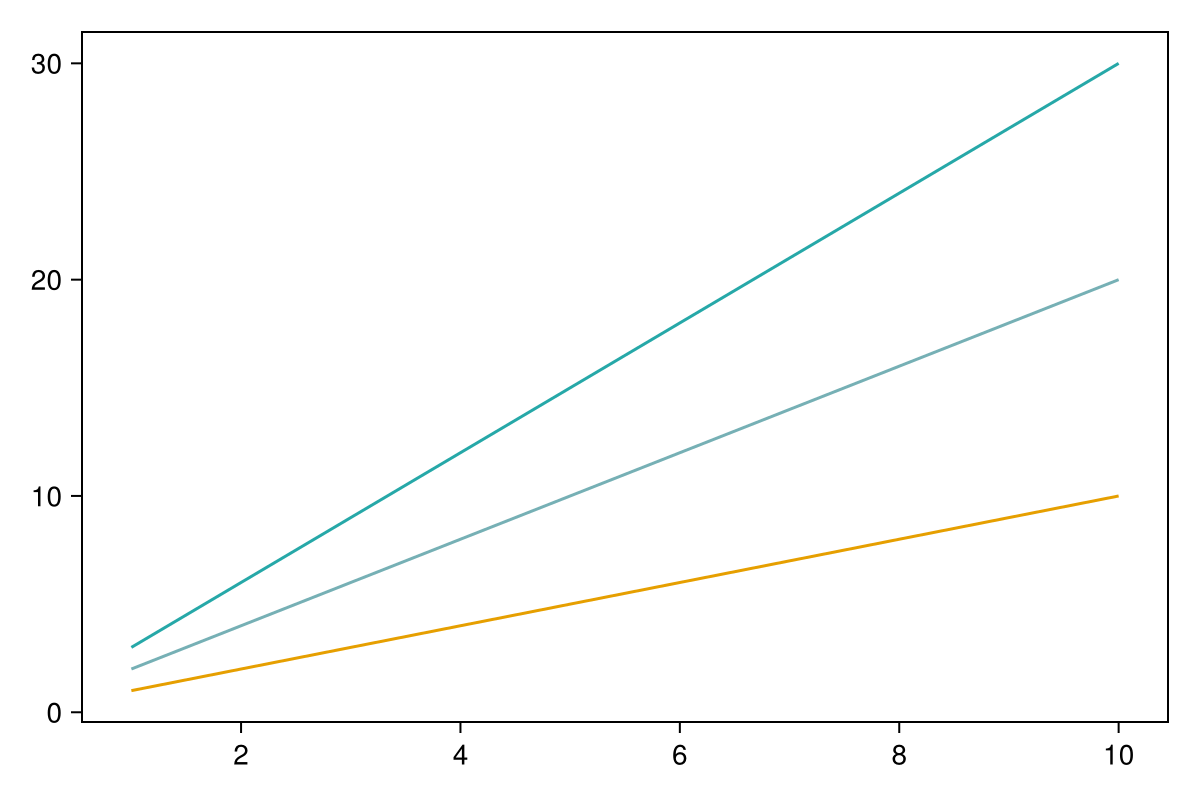
Raster plots
raster creates a new figure, raster! draws into an existing axis. Both accept a population (or stimulus) that records :fire, a NamedTuple of populations such as model.pop (stacked, labelled by name), or a Spiketimes vector. The time window is in ms (0:1s); the axis is in seconds for populations, in ms for a Spiketimes vector. names relabels the populations, other keywords go to scatter!. Above 200 000 spikes the plot is subsampled, with a warning.
using SpikingNeuralNetworks, CairoMakie
SNN.@load_units
E = SNN.IF(N = 80, name = "E")
I = SNN.IF(N = 20, name = "I")
input = SNN.Poisson(N = 100, param = SNN.PoissonParameter(10Hz), name = "input")
inE = SNN.SpikingSynapse(input, E, :ge, conn = (p = 0.2, μ = 3.0))
inI = SNN.SpikingSynapse(input, I, :ge, conn = (p = 0.2, μ = 3.0))
EI = SNN.SpikingSynapse(E, I, :ge, conn = (p = 0.2, μ = 2.0))
IE = SNN.SpikingSynapse(I, E, :gi, conn = (p = 0.2, μ = 5.0))
model = SNN.compose(; E, I, input, inE, inI, EI, IE, silent = true)
SNN.monitor!(model.pop, [:fire])
SNN.sim!(; model, duration = 1s)

fig, ax, plt = SNN.raster(model.pop, 0:1s)        # all populations, new figure

fig2 = Figure()
ax2 = Axis(fig2[1, 1], xlabel = "Time (s)", ylabel = "Neuron")
SNN.raster!(ax2, model.pop.E, 0:500ms)           # one population into an existing axis
fig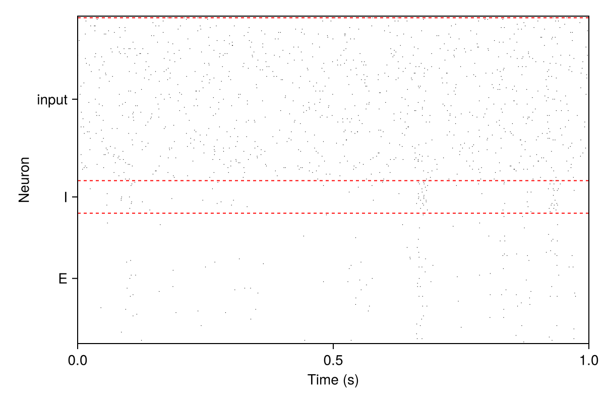
Recorded variables
vecplot and vecplot! plot the time course of any recorded variable (:v, :w, synaptic conductances, ...). The variable must be recorded with monitor!(pop, [sym]). The interpolated record is sampled on interval (ms, default the whole record); neurons selects the neurons, pop_average = true plots the mean (with ribbon = true, also the 20-80 % band), add_spikes = true marks the spikes as 20 mV peaks on the trace. Three-dimensional records (one value per compartment) need sym_id. The x tick labels are in seconds.
using SpikingNeuralNetworks, CairoMakie
SNN.@load_units
E = SNN.IF(N = 5, param = SNN.IFParameter(gl = 10nS, C = 200pF))
stim = SNN.CurrentStimulus(E; param = SNN.CurrentNoise(E; I_base = 300pA))
model = SNN.compose(; E, stim, silent = true)
SNN.monitor!(E, [:v, :fire])
SNN.sim!(; model, duration = 300ms)

fig, ax, plt = SNN.vecplot(E, :v; interval = 0:1:300ms, neurons = 1:2,
                           add_spikes = true, ylabel = "V (mV)")
fig2 = Figure()
ax2 = Axis(fig2[1, 1], ylabel = "V (mV)")
SNN.vecplot!(ax2, E, :v; pop_average = true, ribbon = true)
fig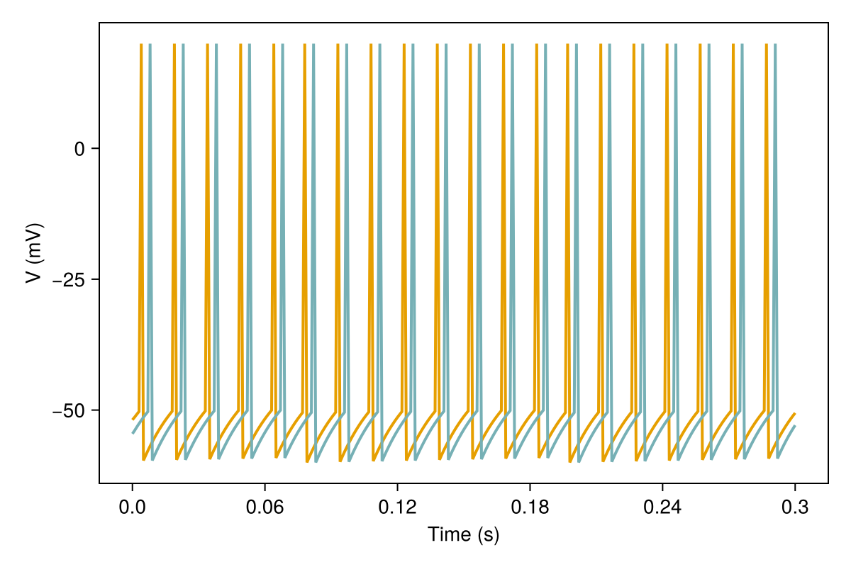
vecplot(P::Array, sym) (one panel per population) and vecplot(p, Any[:v, :w]) (one panel per variable) return a Figure with stacked panels; vecplot(p, [:v, :w]) draws all variables in one axis with their names as legend labels. factor multiplies the trace by a number, by another recorded variable (factor = :g) or by a neurons x time matrix.
STDP kernels
stdp_kernel (new figure) and stdp_kernel! (existing axis) plot the weight change of a long-term plasticity rule as a function of the spike-time difference $\Delta t = t_{post} - t_{pre}$. Each point is a separate two-neuron train! run of 400 ms (stdp_test) measuring one pre/post pair; the default grid has 40 points, so reduce ΔTs for a quick look.
using SpikingNeuralNetworks, CairoMakie
SNN.@load_units
fig = SNN.stdp_kernel(SNN.STDPGerstner(); ΔTs = [-40.0, -20.0, -10.0, -5.0, 5.0, 10.0, 20.0, 40.0])
dw = SNNPlots.stdp_test(SNN.STDPGerstner(); ΔT = 10ms)   # single pairing
fig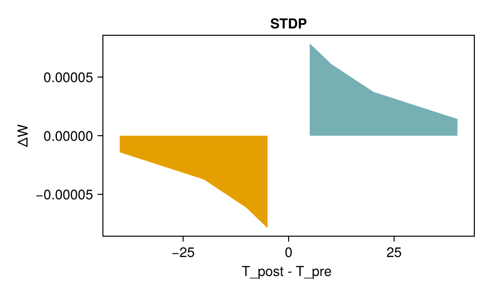
Spatial networks
plot_spatial_connectivity and plot_connection_distances plot the layout and the distance dependence of spatially embedded networks with three populations named :Exc, :PV, :SST. They take the connectivity and configuration objects of a specific spatial-network workflow (fields points, links, network, spatial, or distance histograms ds, rs); see their docstrings for the expected layout. They are not generic plots of an SNNModels model.
API
SNNPlots.SNNPlots — Module
SNNPlotsMakie-based plotting for SNNModels: raster plots (raster, raster!), recorded-variable traces (vecplot, vecplot!), STDP kernels (stdp_kernel, stdp_kernel!, stdp_test) and spatial-network plots (plot_spatial_connectivity, plot_connection_distances).
SNNPlots depends on Makie only; load a Makie backend (using CairoMakie or using GLMakie) to display or save figures. The SNNPlots theme (makie_default!) is applied when the package is loaded.
SNNPlots.okabe_ito_10 — Constant
okabe_ito_10Ten colours sampled uniformly from the Okabe-Ito colour-blind-safe scheme (ColorSchemes.okabe_ito), as a Vector of RGB colours. It is the default Makie colour cycle set by makie_default! and is used by the spatial plots of SNNPlots.
Example
using SpikingNeuralNetworks
c = okabe_ito_10[2]SNNPlots.makie_default! — Method
makie_default!()Apply the SNNPlots Makie theme to the global Makie theme with Makie.set_theme!.
The theme sets: figure size (600, 400); Axis without x and y grid lines; Legend without frame and with label size 10; colour palette okabe_ito_10; Lines and Band cycling through the palette colours.
Since SNNPlots 0.2.10 it is called from SNNPlots.__init__, so it takes effect every time the package is loaded (a top-level call would run only during precompilation and be lost in the user session). Call it again to restore the theme after set_theme!/update_theme! elsewhere. Returns the value of set_theme! (nothing).
Example
using SpikingNeuralNetworks
SNNPlots.makie_default!()SNNPlots.@makie_default — Macro
@makie_defaultBackward-compatible macro form of makie_default!: expands to SNNPlots.makie_default!(), i.e. re-applies the SNNPlots Makie theme. The theme is already applied when SNNPlots is loaded, so the macro is only needed to restore it after another set_theme!. The expansion refers to the name SNNPlots, which must therefore be visible in the calling scope (it is, after using SpikingNeuralNetworks or import SNNPlots).
SNNPlots.raster — Function
raster(spiketimes::Spiketimes, t = nothing; markersize = 1)
raster(P, t = nothing; kwargs...)
Raster plot of spike times in a new Makie figure. Returns a Makie.FigureAxisPlot (destructure it as fig, ax, plt = raster(...)).
Two methods:
raster(spiketimes, t; markersize):spiketimesis aSpiketimes(Vector{Vector{Float32}}, one vector of spike times in ms per neuron, as returned byspiketimes(pop)).tis the time window[t_start, t_end]in ms (default[0, latest spike]). Neuronnis drawn on rown. Spike times are plotted in ms and the axis is labelled "Time (ms)". (Up to SNNPlots 0.2.10markersizewas positional and the label read "Time (s)".)raster(P, t; kwargs...):Pis a population, a stimulus, or aNamedTupleof them (for examplemodel.pop). Creates aFigureand anAxisand callsraster!with the same arguments; see there for the keyword arguments. Time is shown in seconds.
The populations must record spikes: call monitor!(pop, [:fire]) before the simulation. At most 200 000 spikes are drawn; larger sets are randomly subsampled (with a warning) by SNNModels.resample_spikes.
Example
using SpikingNeuralNetworks
SNN.@load_units
E = SNN.Poisson(N = 50, param = SNN.PoissonParameter(10Hz))
SNN.monitor!(E, [:fire])
SNN.sim!([E]; duration = 1s)
fig, ax, plt = SNN.raster(E, 0:1s)       # population method, time axis in s
fig2, ax2, plt2 = SNN.raster(SNN.spiketimes(E)) # Spiketimes methodSNNPlots.raster! — Function
raster!(ax::Axis, spiketimes::Spiketimes, t = nothing; markersize = 1, order = nothing, kwargs...)
raster!(ax, P, t = nothing; interval = nothing, populations = nothing, names = nothing,
        every = 1, markersize = 1, order = [], kwargs...)
Draw a raster plot into the existing Makie axis ax and return the scatter plot object.
Spiketimes method: spiketimes holds one vector of spike times (ms) per neuron; t is the window [t_start, t_end] (ms, default [0, latest spike]); order is an optional permutation of the neurons (neuron order[k] is drawn on row k); remaining kwargs are passed to Makie.scatter!. Times are plotted in ms.
Population method: P is a population/stimulus or a NamedTuple of them; populations are stacked vertically, separated by red dashed lines, and labelled on the y axis with the first 10 characters of their name. Keyword arguments:
torinterval: time window in ms (a range or a two-element vector);thas precedence. The x axis is in seconds (spike times are divided bys).populations: if given,Pmust be a single population andpopulationsa vector of index vectors; each index set is drawn as a separate group, labelled withnames(default"pop_i"). Withoutpopulations,names(if given) labels the populations, otherwise theirnamefields are used.every = 1: draw one spike out ofevery.markersize = 1: marker size.order = []: neuron order passed to the per-population raster.- other
kwargsare passed toMakie.scatter!.
Requires a :fire record on every population (monitor!(pop, [:fire])). The y-limits are set on ax. (Up to SNNPlots 0.2.10 they were set on the current axis, names was ignored without populations, the extra kwargs were dropped, and raster! was not exported.)
Example
using SpikingNeuralNetworks, CairoMakie
SNN.@load_units
E = SNN.Poisson(N = 40, param = SNN.PoissonParameter(10Hz), name = "E")
I = SNN.Poisson(N = 10, param = SNN.PoissonParameter(20Hz), name = "I")
SNN.monitor!([E, I], [:fire])
SNN.sim!([E, I]; duration = 1s)
fig = Figure()
ax = Axis(fig[1, 1], xlabel = "Time (s)")
raster!(ax, (; E, I), 0:1s)SNNPlots.vecplot! — Method
vecplot!(ax, p, sym; neurons = nothing, pop_average = false, interval = nothing, r = nothing,
         sym_id = nothing, factor = 1.0f0, add_spikes = false, variables = nothing, lw = 2,
         color = nothing, ribbon = false, label = nothing, kwargs...)
vecplot!(ax, p, sym::Symbol, interval::AbstractRange; kwargs...)
Draw the recorded variable sym of p into the Makie axis ax; returns the last lines! plot.
The record is read with SNNModels.record(p, sym; variables, range = true), which returns an interpolated record and its time range.
Keyword arguments:
interval(orr;intervalhas precedence): time range in ms at which the interpolated record is sampled. Default: from the first to the last recorded time in steps of 1 ms. An error is thrown if the range exceeds the recorded time.neurons: neuron indices (anIntor a collection); default all.pop_average = false: plot the mean over the selected neurons.ribbon = false: withpop_average = true, also draw a band between the 20th and 80th percentiles across neurons.sym_id: required when the record is three-dimensional (e.g. one value per dendritic compartment): index of the second dimension to plot.factor = 1.0f0: scalar multiplying the trace, or theSymbolof another recorded variable ofp(sampled on the same times) or aneurons x timematrix to multiply it point-wise. (Up to SNNPlots 0.2.10 theSymbolandMatrixforms threw.)add_spikes = false: set the trace to 20 mV at the first sample after every spike (needs a:firerecord).variables: forwarded torecord(selects variables of a nested record).lw = 2: line width;color: line colour (default: cycle through the theme palette by neuron index);label: legend label (converted withstring).- other
kwargsare passed toMakie.lines!.
x data are in ms; the six x ticks are relabelled in seconds.
Example
using SpikingNeuralNetworks, CairoMakie
SNN.@load_units
E = SNN.IF(N = 5, param = SNN.IFParameter(gl = 10nS, C = 200pF))
SNN.monitor!(E, [:v])
stim = SNN.CurrentStimulus(E; param = SNN.CurrentNoise(E; I_base = 300pA))
model = SNN.compose(; E, stim)
SNN.sim!(; model, duration = 200ms)
fig = Figure()
ax = Axis(fig[1, 1], ylabel = "V (mV)")
SNN.vecplot!(ax, E, :v; pop_average = true, ribbon = true)SNNPlots.vecplot — Method
vecplot(p, sym::Symbol; kwargs...)
vecplot(p, syms::Vector{Symbol}; interval = nothing, ylabel = "", title = "", kwargs...)
vecplot(p, sym, interval::AbstractRange; kwargs...)
Plot the recorded time course of the variable(s) sym of the population (or connection, stimulus) p in a new Makie figure; returns a Makie.FigureAxisPlot.
The variable must have been recorded with monitor!(p, [sym]) before the simulation. One line is drawn per neuron (or one line for the population mean with pop_average = true); every keyword argument not listed here is forwarded to vecplot! (neurons, pop_average, r, sym_id, factor, add_spikes, variables, lw, color, ribbon, ...).
interval: time range in ms (e.g.0:1:1000msor0:1s); default: the whole record.ylabel,title: axis labels.
The x axis data are in ms and the tick labels are shown in seconds.
vecplot(p, syms::Vector{Symbol}) draws all symbols in one axis. vecplot(P::Array, sym::Symbol) (one panel per population) and vecplot(p, syms::Array) with a vector that is not a Vector{Symbol} (e.g. Any[:v, :w], one panel per symbol) stack the panels vertically and return the Figure. (Up to SNNPlots 0.2.10 they called the Plots.jl plot(...; layout) API and failed with Makie; the legend label of each line was always "nothing".)
Example
using SpikingNeuralNetworks
SNN.@load_units
E = SNN.IF(N = 5, param = SNN.IFParameter(gl = 10nS, C = 200pF))
SNN.monitor!(E, [:v])
stim = SNN.CurrentStimulus(E; param = SNN.CurrentNoise(E; I_base = 300pA))
model = SNN.compose(; E, stim)
SNN.sim!(; model, duration = 200ms)
fig, ax, plt = SNN.vecplot(E, :v, interval = 0:1:200ms, neurons = 1:2, ylabel = "V (mV)")SNNPlots.stdp_kernel! — Method
stdp_kernel!(ax, stdp_param; ΔTs = vcat(range(-200, -0.1, 20), range(0.1, 200, 20)), fill = false, kwargs...)Plot the STDP kernel of the plasticity rule stdp_param into the Makie axis ax.
For each ΔT in ΔTs (ms, t_post - t_pre) the weight change is measured with stdp_test (a full two-neuron train! run per point, run in parallel with Threads.@threads). The negative and positive branches are drawn as two lines with a band down to zero. fill and kwargs are accepted but unused. Returns the last band! plot.
Arguments
ax: a MakieAxis.stdp_param: a long-term plasticity parameter (LTPParameter), e.g.STDPGerstner().ΔTs: spike-time differences in ms (default 20 points in [-200, -0.1] and 20 in [0.1, 200]).
Example
using SpikingNeuralNetworks, CairoMakie
SNN.@load_units
fig = Figure()
ax = Axis(fig[1, 1], xlabel = "Δt (ms)", ylabel = "ΔW")
SNN.stdp_kernel!(ax, SNN.STDPGerstner(); ΔTs = [-20.0, -5.0, 5.0, 20.0])SNNPlots.stdp_kernel — Method
stdp_kernel(stdp_param; kwargs...)Create a 500x300 Makie Figure with an axis titled "STDP" (x: T_post - T_pre, y: ΔW), draw the kernel of stdp_param with stdp_kernel! (same keyword arguments) and return the Figure.
Example
using SpikingNeuralNetworks
SNN.@load_units
fig = SNN.stdp_kernel(SNN.STDPGerstner(); ΔTs = [-20.0, -5.0, 5.0, 20.0])SNNPlots.stdp_test — Method
stdp_test(stdp_param; ΔT)Measure the weight change produced by the long-term plasticity rule stdp_param (any LTPParameter, e.g. STDPGerstner()) for a single pre/post spike pair with time difference ΔT = t_post - t_pre (ms).
Builds a presynaptic and a postsynaptic Identity neuron, each driven by its own SpikeTimeStimulusIdentity: the presynaptic neuron spikes at 200 ms and the postsynaptic one at 200ms + ΔT. A SpikingSynapse pre -> post with initial weight 1 and LTPParam = stdp_param is trained with train! for 400 ms at dt = 0.1ms (plasticity only runs under train!). The synapse transmits into a dummy buffer, so it does not make the postsynaptic neuron fire: exactly one pre/post pair is measured. Returns the weight change W - 1.
Up to SNNPlots 0.2.10 both neurons belonged to one Identity population and the measured synapse also drove the postsynaptic neuron, which emitted an extra spike one step after the presynaptic spike: every measured change contained an extra causal pair at Δt ≈ 0.1 ms (for STDPGerstner(): +1.6e-4 at ΔT = 10ms and +3.9e-5 instead of a depression at ΔT = -10ms).
Example
using SpikingNeuralNetworks
SNN.@load_units
dw = SNNPlots.stdp_test(SNN.STDPGerstner(); ΔT = 10ms)SNNPlots.plot_connection_distances — Method
plot_connection_distances(fig; ds, rs, probability = true)Plot the distribution of connection distances from the populations :Exc, :PV, :SST to the :Exc population (Makie). The distance histograms must be computed beforehand.
Generates two plots:
fig[1, 1]: grouped bar plot of the normalised connection counts per distance bin ("Conn. density").fig[1, 2](only ifprobability = true): the counts divided by the squared bin edge and normalised, as a proxy of the connection probability per unit area ("Conn. probability").
Arguments
fig: the MakieFigureto plot into.ds: dictionary of binned connection counts, keyed byname(pre, :Exc)for eachprein(:Exc, :PV, :SST).rs: the bin edges (a range in the library length unit, cm); the x axis is shown in mm (rs * 10).probability::Bool = true: also draw the probability panel.
Returns the result of the last barplot! call.
SNNPlots.plot_spatial_connectivity — Method
plot_spatial_connectivity(fig, connectivity, config; post = :Exc, n0 = rand(1:20),
                          do_arrows = true, rotation = :horizontal, xlabel = "",
                          ylabel = "", do_legend = true)
Visualize the spatial layout of three neuronal populations and their connections to a single postsynaptic neuron (Makie).
Plots all neurons of the populations :Exc, :PV, :SST (hard-coded names, colours okabe_ito_10[[8, 2, 3]], markers triangle/circle/hexagon). For the postsynaptic neuron n0 of population post, highlights all presynaptic neurons connected to it (entries equal to 1 in the adjacency matrices) and draws lines from them to n0, which is marked with a cross.
This function is tied to a specific spatial-network configuration layout and is not a generic SNNModels plot.
Arguments
fig: Makie figure orGridLayout; the axis is placed atfig[1:2, 1:2], the legend atfig[0, 1:2].connectivity: object with fieldspoints(per-population vectors of neuron coordinates) andlinks(adjacency matrices keyed bySymbol(str_name(pre, post, compartment)), indexed[post, pre]).config: configuration withnetwork(fieldsrecurrence.connections,Npop,targets) andspatial(fieldgrid_size).post::Symbol = :Exc: postsynaptic population.n0::Int = rand(1:20): index of the postsynaptic neuron.do_arrows::Bool = true: draw connection lines.rotation::Symbol = :horizontal::horizontal(x = first coordinate) or:vertical(swap x and y).xlabel,ylabel: labels of the x-data and y-data axes (default""), swapped automatically whenrotation = :vertical.do_legend::Bool = true: draw the legend.
Ticks are placed at range(0, 0.1, 5) and labelled 0, 0.25, ..., 1 (coordinates are assumed to lie in [0, 0.1], i.e. 1 mm in the library unit system).
Returns
The Axis if do_legend = true; otherwise the tuple (ax, legend_info) where legend_info is a NamedTuple with the legend elements, labels and placement options, to build the legend elsewhere.